Moving window analysis, sometimes referred to as focal analysis, is the process of calculating a value for a specific neighborhood of cells in a given raster. Typical functions calculated across the neighborhood are sum, mean, min, max, range, etc.
However, there are some key differences to keep in mind if you are using continuous vs. discrete data and/or applying a rectangular or circular moving window. These are fairly straightforward exercises in a GIS, but they become a bit more complex when executed in R (especially when applying a circular moving window to discrete data). Below I outline examples of these four workflows in R.
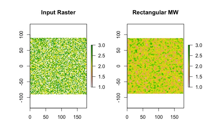
1. Apply Rectangular Moving Window to Continuous Data
library(raster)
set.seed(12345)
# create raster data
r <- raster(nrows = 120, ncol = 120, xmn=0)
r[] <- sample(3, ncell(r), replace=TRUE)
r #note: pixel resolution is 1.5 x 1.5

#set margins for plots
par(mfrow=c(1,2), oma=c(0,1, 0, 1))  # all sides have 3 lines of space

###
#1 apply rectangular moving window to continuous data
###
# 3x3 mean filter - rectangle
r.R3 <- focal(r, w=matrix(1/9,nrow=3,ncol=3), na.rm=FALSE) #the default is to not consider NAs
plot(r, main ="Input Raster") #plot orig
plot(r.R3, main="Rectangular MW") #plot 3x3 moving window
#####
#####
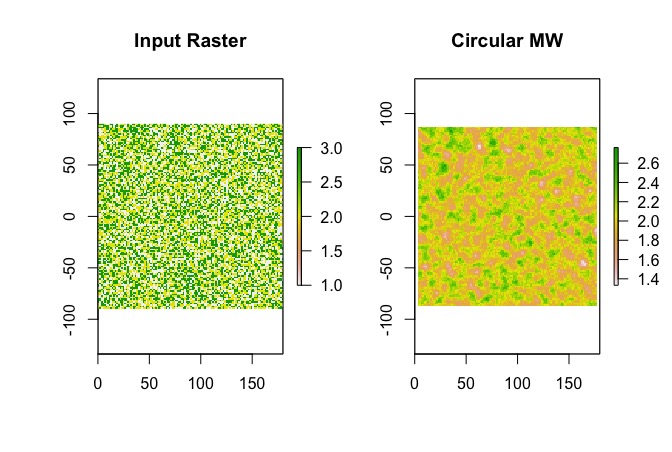
2. Apply Circular Moving Window to Continuous Data
###
#2 apply circular moving window to continuous data
###
#set the focal weight, since we are using a circle, set number to the radius of the circle (in units of CRS)
#cell resolution is 1.5 x 1.5
fw <- focalWeight(r, 4, type='circle')
#have a look at the shape of the moving window
fw
# apply moving window
r.C4<-focal(r, w=fw, na.rm=TRUE)
plot(r, main ="Input Raster") #plot original
plot(r.C4, main="Circular MW")
####
####
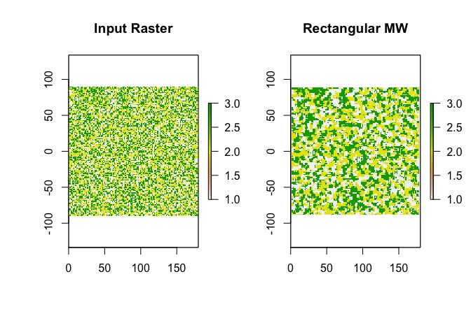
3. Apply Rectangular Moving Window to Discrete Data
###
#3 apply rectangular moving window to discrete data (e.g. integer)
###
# 3x3 moving window; note, function is set to modal, so we will find the mode or count of each number...this essentially treats it as categorical
r.CAT.R3<-focal(r, w=matrix(1,3,3), fun=modal)
plot(r) #plot original
plot(r.CAT.R3)
####
####
4. Apply Circular Moving Window to Discrete Data
###
#4 apply circular moving window to discrete data (e.g. integer)
###
#set up window
fw <- ceiling(focalWeight(r, 5, type='circle'))#for integer output; type = circle indicates that d is in the units of the CRS
fw #take a look at the architecture of the moving window
#I highly recommend you set the zero's in the moving window to NA. If not, zero's can be added into your discrete data output under certain sizes/shapes of moving windows. Check the legend of the output data to identify if a zero has been introduced.
fw[fw==0]<-NA
fw
#apply focal fxn
r.CAT.C5<-focal(r, w=fw, fun=modal, na.rm=TRUE)
plot(r, main ="Input Raster") #plot original
plot(r.CAT.C5, main="Circular MW")
#####
#####
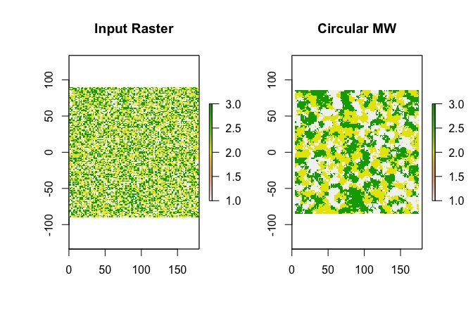
When doing analysis #4 in R, I highly recommend you set the zero’s in the moving window to NA. If not, zero’s can be added into your discrete data output under certain sizes/shapes of moving windows. Check the legend of the output data to identify if a zero has been introduced.
Top image: Milano Centrale Railway Station, Lombardy, Italy.