Here is an excerpt from a recent lecture on GLM binomial models that went over pretty well with my students. We’ll run a basic multi-variate logistic model, then calculate the probability prediction. Then, we’ll add a second independent variable to the model, calculate the probability for each predictor variable (while holding the other constant at it’s mean), and plot the two curves.
Probability of passing an exam
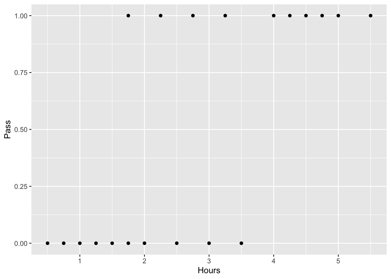
A group of 20 students spends between 0 and 6 hours studying for an exam. How does the number of hours spent studying affect the probability of the student passing the exam?
The reason for using logistic regression for this problem is that the values of the dependent variable, pass and fail, while represented by “1” and “0”. If the problem was changed so that pass/fail was replaced with the grade 0–100 (cardinal numbers), then simple regression analysis could be used.Let’s create a dataframe from two vectors: Pass (1= Pass, 0 = Fail) and Hours (# of hours of study):
Hours<- c(0.50, 0.75, 1.00, 1.25,   1.50, 1.75, 1.75,   2.00, 2.25, 2.50, 2.75, 3.00, 3.25, 3.50, 4.00, 4.25,   4.50, 4.75, 5.00,   5.50)
Pass<-  c(0, 0, 0, 0,   0,  0, 1, 0, 1, 0, 1, 0, 1, 0, 1, 1, 1, 1, 1, 1)
study.df<-data.frame(Hours, Pass)

library(tidyverse)
ggplot(study.df, aes(x=Hours, y=Pass)) + geom_point() #plot it
Run the model:
glm.logit <- glm(Pass ~ Hours, data = study.df, family = binomial) # family = binomial required for logistic regression
summary(glm.logit)

##
## Call:
## glm(formula = Pass ~ Hours, family = binomial, data = study.df)
##
## Deviance Residuals:
##      Min        1Q    Median        3Q       Max
## -1.70557  -0.57357  -0.04654   0.45470   1.82008
##
## Coefficients:
##             Estimate Std. Error z value Pr(>|z|)
## (Intercept)  -4.0777     1.7610  -2.316   0.0206 *
## Hours         1.5046     0.6287   2.393   0.0167 *
## ---
## Signif. codes:  0 '***' 0.001 '**' 0.01 '*' 0.05 '.' 0.1 ' ' 1
##
## (Dispersion parameter for binomial family taken to be 1)
##
##     Null deviance: 27.726  on 19  degrees of freedom
## Residual deviance: 16.060  on 18  degrees of freedom
## AIC: 20.06
##
## Number of Fisher Scoring iterations: 5
Interpretation of the output
The output indicates that hours studying is significantly associated with the probability of passing the exam (p = 0.0167).
The parameter estimates are similar to linear regression.
B0 = − 4.0777 and B1= 1.5046
We can write the formula the same way as in linear regression: y ~ -4.08 + 1.51 x
However, in logistic regression, this equation will estimate the log odds of passing the exam.To calculate the odds of passing the exam we would use the equation: exp(-4.08 + 1.51 x)
However, using the equation in the image above, we can covert the odds to the probability of passing the exam: p = 1/(1+exp(-(1.5046*x-4.0777)))
Now we’ll plot the fitted the probability as a function of the linear predictor:
#get the predicted probs for each x value
study.df$Prob <- predict(glm.logit, type = 'response')

ggplot(study.df, aes(x=Hours, y=Prob)) +
  geom_point() +
  geom_smooth(method = "glm", method.args = list(family = "binomial"), se = FALSE, alpha=0.3)
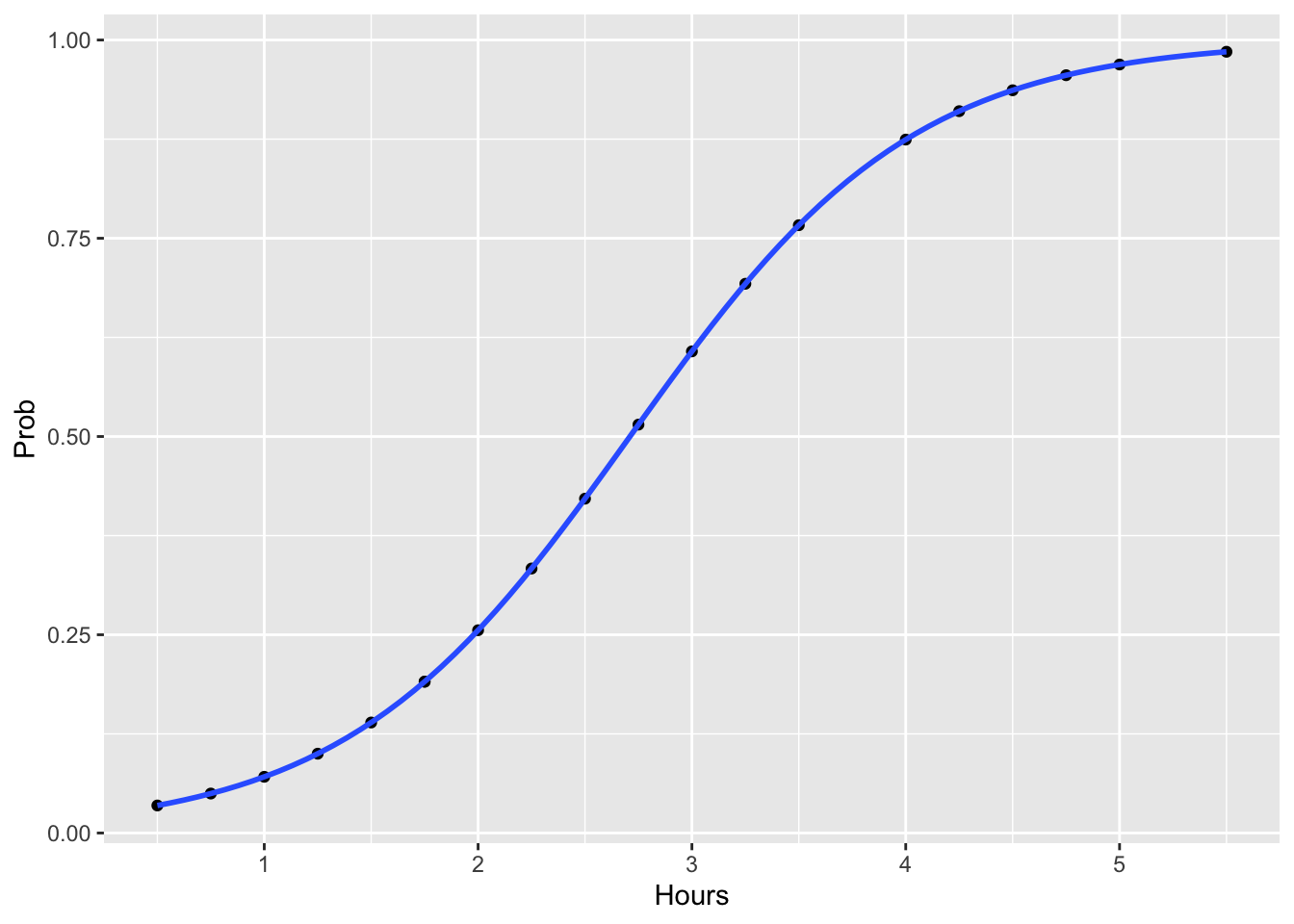
Now that we’ve taken the time to convert the response variable to a meaningful scale, it is very straightforward to interpret.
Psuedo R2
When analyzing data with a logistic regression (or any GLM for that matter), an equivalent statistic to R-squared does not exist. The model estimates from a logistic regression are maximum likelihood estimates arrived at through an iterative process. They are not calculated to minimize variance, so the OLS approach to goodness-of-fit does not apply. However, to evaluate the goodness-of-fit of logistic models, several pseudo R-squareds have been developed. These are “pseudo” R-squareds because they look like R-squared in the sense that they are on a similar scale, ranging from 0 to 1, with higher values indicating better model fit.
We’ll use the pscl package:
#compute various pseudo-R2 measures using pscl library
library(pscl)
pR2(glm.logit) #see r2ML for the Maximum likelihood pseudo r-squared
There are a number of ways to assess logistic model fit in addition to psuedo-R2 such as the Likelihood Ratio Test and the Hosmer-Lemeshow Test. There are also several ways to assess individual model predictors such as the Wald Test and Variable importance. There are a number of ways to assess validation of predicted values when developing models for prediction (e.g. species distribution models) such as classification rate, ROC Curve, and k-fold cross validation.
Multivariate Logistic Regression
Multivariate logistic regression operates the same way as the example above, however, it includes two or more independent variables. Let’s add another variable to our previous example:
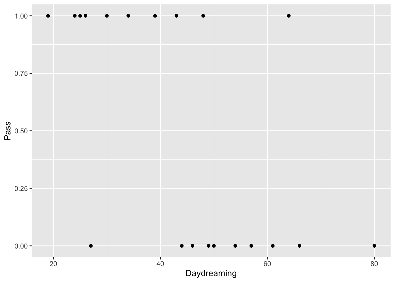
Let’s overwrite the dataframe we created earlier. We’ll create a dataframe from three vectors this time: Pass (1= Pass, 0 = Fail), Hours (# of hours of study) and Daydreaming (# of minutes daydreaming in class)
Hours<- c(0.50, 0.75, 1.00, 1.25,   1.50, 1.75, 1.75,   2.00, 2.25, 2.50, 2.75, 3.00, 3.25, 3.50, 4.00, 4.25,   4.50, 4.75, 5.00,   5.50)
Pass<-  c(0, 0, 0, 0,   0,  0, 1, 0, 1, 0, 1, 0, 1, 0, 1, 1, 1, 1, 1, 1)
Daydreaming<-c(50, 49, 46, 80, 27, 57, 25, 66, 30, 61, 43, 44, 26, 54, 48, 34, 24, 39, 64, 19)
study.df<-data.frame(Hours, Pass, Daydreaming)

ggplot(study.df, aes(x=Daydreaming, y=Pass)) + geom_point() #plot the new variable daydreaming vs. pass/fail
Run the model:
glm.logit2 <- glm(Pass ~ Hours + Daydreaming, data = study.df, family = binomial,
                  control = list(maxit = 50)) # family = binomial required for logistic regression

summary(glm.logit2)

##
## Call:
## glm(formula = Pass ~ Hours + Daydreaming, family = binomial,
##     data = study.df, control = list(maxit = 50))
##
## Deviance Residuals:
##      Min        1Q    Median        3Q       Max
## -1.29052  -0.00021   0.00000   0.02102   1.67187
##
## Coefficients:
##             Estimate Std. Error z value Pr(>|z|)
## (Intercept)   3.7429     4.5428   0.824    0.410
## Hours         8.0012     5.5968   1.430    0.153
## Daydreaming  -0.6246     0.4277  -1.460    0.144
##
## (Dispersion parameter for binomial family taken to be 1)
##
##     Null deviance: 27.7259  on 19  degrees of freedom
## Residual deviance:  5.6559  on 17  degrees of freedom
## AIC: 11.656
##
## Number of Fisher Scoring iterations: 10
For the purposes of this exercise, do not worry about the significance of the p-values.
Interpretation of the output
The interpretation of the output is similar to multiple linear regression in that you interpret X1 while holding all of the other independent variables constant. However, it’s a bit trickier in logistic regression because you need to convert the log odds to a probability scale like we did in the logistic regression example above.
I find it very helpful to calculate the probability predictions for y while adjusting the values of X1 while holding all other independent variables constant at their respective mean (instead of 1 or some other arbitrary value). You could plug in a bunch of successive values for X1 while holding X2 constant to get a sense of how X1 changes the probability in y. Or better yet, you can calculate a new column in your dataframe for the estimated probability of each value of X1 using the mean of X2 with the formula: 1/(1+exp(-(B0 + B1X1 + B2MeanX2))
Repeat this process for each independent variable. This can be accomplished using the mutate function and the pipe operator in just a few lines of code.Then you will be able to plot the fitted probability for each independent variable just as you did previously in the lesson. However, you will have one graph for each independent variable that will give you a clear indication how a change in one unit of X1 (and X2, etc.) will affect the probability in y.
Let’s illustrate this process:
#get the means of each predictor variable and write to a variable
mean.Hours<-mean(study.df$Hours)
mean.Daydreaming<-mean(study.df$Daydreaming)
Next, we’ll write the dataset to a new dataframe and calculate the probabilities in the process.
#manipulate the dataset:
#calculate the prob for hours of study when daydreaming is held constant at mean daydreaming
##calculate the prob for daydreaming in class when hours are held constant at mean hours
study.df2 <- study.df %>%
  mutate(prob.Hours = 1/(1+exp(-(3.7429 + 8.0012*Hours -0.6246*mean.Daydreaming)))) %>%  #hold Daydreaming constant
  mutate(prob.Daydreaming = 1/(1+exp(-(3.7429 + 8.0012*mean.Hours -0.6246*Daydreaming)))) #hold hours constant
Next we will create a graph similar to what we did earlier, but we will need to create two, one for each predictor variable.
#plot area probabilities when Daydreaming is held constant
g.prob.Hours<-ggplot(study.df2, aes(x=Hours, y=prob.Hours)) +
  geom_point() +
  geom_smooth(method = "glm", method.args = list(family = "binomial"), se = FALSE, alpha=0.3)+
  labs(x = "Hours of Study",
       y = "Probability of Pasing Exam")+
  ggtitle("Prob of Passing with Daydreaming held constant:") +
  theme(plot.title = element_text(size=8))+
  theme(axis.title = element_text(size=10))

#plot isolation probabilities when hours are held constant
g.prob.Daydreaming<-ggplot(study.df2, aes(x=Daydreaming, y=prob.Daydreaming)) +
  geom_point() +
  geom_smooth(method = "glm", method.args = list(family = "binomial"), se = FALSE, alpha=0.3)+
  labs(x = "Minutes of Daydreaming in Class",
       y = "Probability of Pasing Exam")+
  ggtitle("Prob of Passing with Hours held constant:") +
  theme(plot.title = element_text(size=8))+
  theme(axis.title = element_text(size=10))

# now put the two graphs together
library(gridExtra)
grid.arrange(g.prob.Hours, g.prob.Daydreaming, ncol=2, widths = c(6,6))
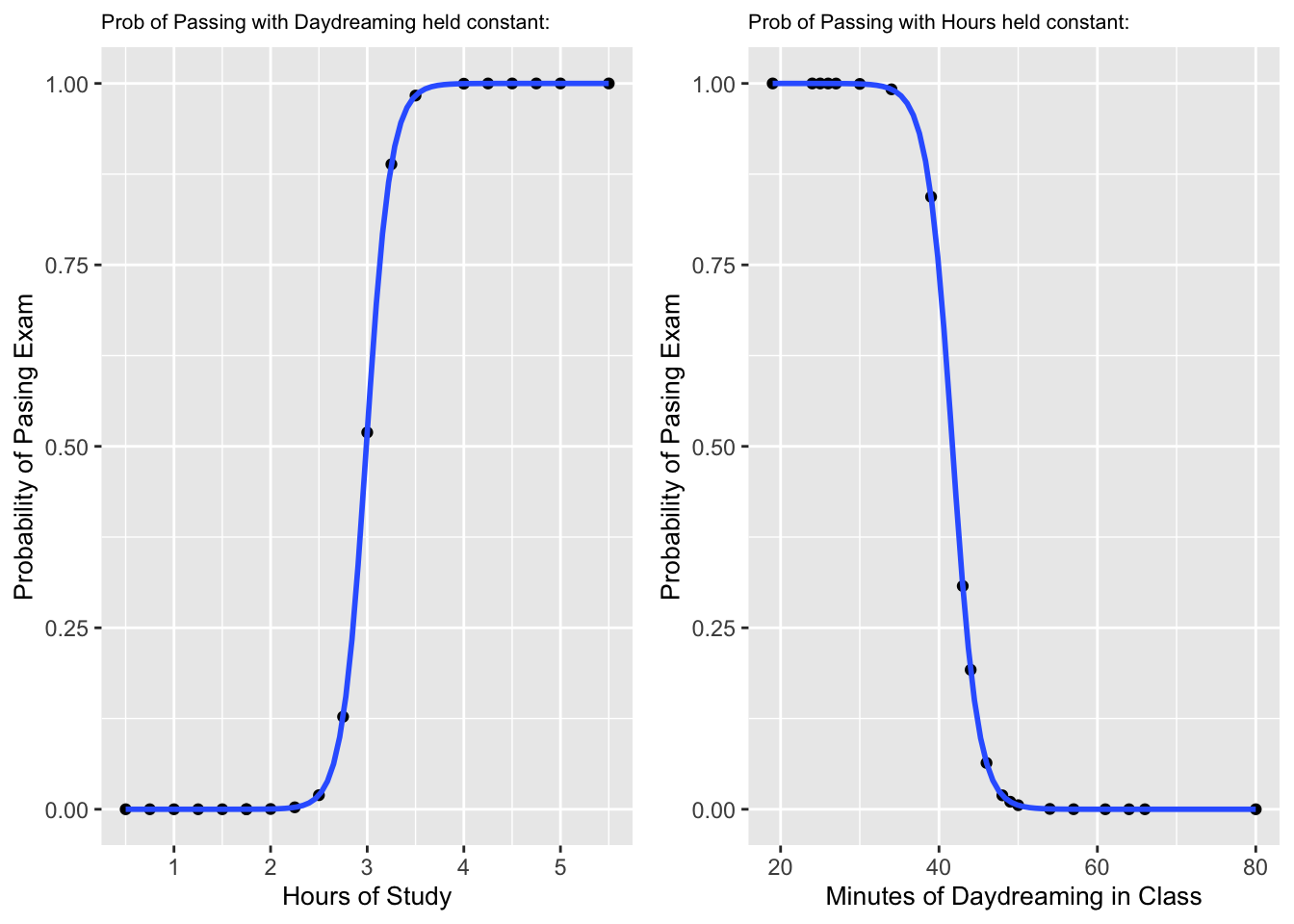
Once we plot the two predicted probability curves together, we can fully appreciate what the model tells us:
- If you daydream an average amount of time, you will need to study over three hours to pass the exam
- If you study the average amount of time, then you will want to make sure you do not daydream more than 40 minutes during class time if you expect to pass the exam.