I frequently benefit from notes that others have posted regarding workflows in R. Recently I ran into some challenges working with raster data while writing code for species distribution modeling. Although some of the information is already out there, I decided to wrap it together here and add a little context. Like everything I do in R, there are probably more efficient ways to accomplish these tasks, but I hope this is helpful.
In this example, I am working with the outputs of predictive habitat distribution models of two forest cover types developed using logistic regression. Assume a raster is a surface indicating probability of occurrence (0-1) for a given cover type and only one cover type can be present for any given pixel. If a pixel is predicted to contain both forest types, the values from each model above the presence threshold need to be linearly rescaled from 0 to 1. Then the cover type with the highest occurrence probability will be assigned to the pixel.
####load the required packages
library(raster)
library(rgdal)
Rescale raster cell values between 0 and 1. The function below uses cellStats, so the entire range of values are considered.
# generic method to rescale a raster
#load raster
r1<-raster("base_raster.img")

#fxn to rescale cell values between 0 and 1
rasterRescale<-function(r){
  ((r-cellStats(r,"min"))/(cellStats(r,"max")-cellStats(r,"min")))
}

#run the fxn
r2<-rasterRescale(r1)
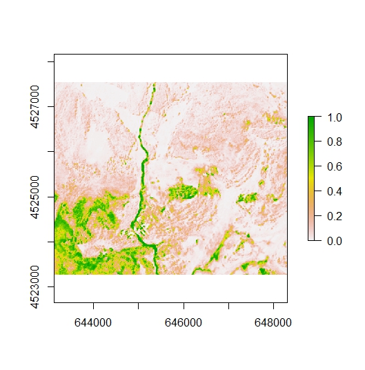
plot(r2)

The function above is not particularly helpful in our situation since we only want to rescale the data above a model selected threshold. We must first reclassify the data below the threshold (e.g. 0.6). In the example below, values of 0 could be reclassified to NA, but in my workflow it’s helpful to set values to 0 so the raster can be incorporated into raster math calculations later on.
#reclassify cell values
#reclassify values below 0.6 to 0; retain cell values above 0.6
r2[r2<=0.6]=0
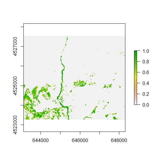
plot(r2)

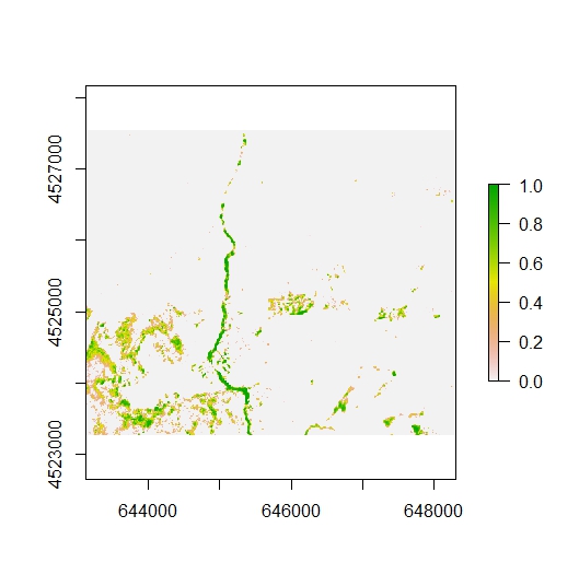
Now we can rescale the data above the threshold from 0 to 1. Compare the differences between the map above with the one below.
#fxn to rescale values between 0 and 1, but rmin and rmax must be specified
rasterRescale.Set<-function(r, rmin, rmax){
  ((r-rmin)/(rmax-rmin))
}

#run fxn to rescale raster; rmin=0.6; rmax=1
r3<-rasterRescale.Set(r2, 0.6, 1)
#ensure minimum values are set to 0
r3[r3<=0]=0
plot(r3)

Once each raster is rescaled accordingly, we need to determine which raster has a higher value for a given cell and assign a new value accordingly. This is a straightforward exercise in ArcGIS, but it is a bit more complicated in R.
In my example, one would want to identify the pixels where both species are predicted to occur. I won’t go into that step here, as the workflow below only addresses those pixels where there are probability values for each cover type.
#assume raster r5 and r6 have a range of values that overlap
#r5 rmin=0.35, rmax=1
#r6 rmin=0.6, rmax=1
#determine which cell value is higher, assign 1 if r5, assign 2 if r6, if 0, assign a 0 again

#returns all values of a Raster* object as a matrix
as.matrix(r5)
as.matrix(r6)

#create an empty raster r7 that matches the extent of the other rasters
r7<-raster(ncol=518, nrow=428, xmn=643128.9, xmx=648308.9, ymn=4523269, ymx=4527549)
projection(r7)="+proj=utm +zone=12 +ellps=WGS84 +units=m +no_defs" #assign projection to match

#fxn to execute a conditional statement
Con=function(condition, trueValue, falseValue){
  return(condition * trueValue + (!condition)*falseValue)
}

#create a matrix m and execute conditional statement
m = as.matrix(Con(r5>r6,1,Con(r5<r6, 2, 0))) #if r5<r6, assign value of 1, else value of 2

#assign values of matrix m to raster r7
values(m)=r7

#the raster r7 contains a value of 1 if r5 pixel had a higher value, 2 if r6 had a higher value and 0 if both input rasters had a value of 0.
Now the raster r7 can be used to overwrite the value of a pixel in an ensemble model where both cover types are predicted to occur. Since pixels where only one cover type were predicted to occur are zeroed out, raster r7 can be incorporated into the ensemble model through a basic raster math calculation.
Literature Cited
- Assal, T., Anderson, P., Sibold, J., 2015. Mapping forest functional type in a forest-shrubland ecotone using SPOT imagery and predictive habitat distribution modelling. Remote Sensing Letters. 6, 755–764.
Top image: Generally what my desk looks like at any given time.
